Kleiber's law () is one of those “laws” of nature that is both derived from, and seems to fit quite well with, empirical data. It applies to most animals, including humans. The law is roughly summarized through the equation below, where E = energy expenditure at rest per day, and M = body weight in kilograms.
Because of various assumptions made in the original formulation of the law, the values of E do not translate very well to calories as measured today. What is important is the exponent, and what it means in terms of relative increases in weight. Since the exponent in the equation is 3/4, which is lower than 1, the law essentially states that as body weight increases animals become more efficient from an energy expenditure perspective. For example, the energy expenditure at rest of an elephant, per unit of body weight, is significantly lower than that of a mouse.
The difference in weight does not have to be as large as that between an elephant and a mouse for a clear difference in energy expenditure to be noticed. Moreover, the increase in energy efficiency predicted by the law is independent of what makes up the weight; whether it is more or less lean body mass, for example. And the law is very generic, also applying to different animals of the same species, and even the same animal at different developmental stages.
Extrapolating the law to humans is quite interesting. Let us consider a person weighing 68 kg (about 150 lbs). According to Kleiber's law, and using a constant multiplied to M to make it consistent with current calorie measurement assumptions (see Notes at the end of this post), this person’s energy expenditure at rest per day would be about 1,847 calories.
A person weighing 95 kg (about 210 lbs) would spend 2,374 calories at rest per day according to Kleiber's law. However, if we were to assume a linear increase based on the daily calorie expenditure at a weight of 68 kg, this person weighing 95 kg would spend 2,508 calories per day at rest. The difference of approximately 206 calories per day is a reflection of Kleiber's law.
This difference of 206 calories per day would translate into about 23 g of extra body fat being stored per day. Per month this would be about 688 g, a little more than 1.5 lbs. Not a negligible amount. So, as you become obese, your body becomes even more efficient on a weight-adjusted basis, from an energy expenditure perspective.
One more roadblock to go from obese to lean.
Now, here is the interesting part. It is unreasonable to assume that the extra mass itself has a significantly lower metabolic rate, with this fully accounting for the relative increase in efficiency. It makes more sense to think that the extra mass leads to systemic adaptations, which in turn lead to whole-body economies of scale (). In existing bodies, these adaptations should happen over time, as long-term compensatory adaptations ().
The implications are fascinating. One implication is that, if the compensatory adaptations that lead to a lower metabolic rate are long term, they should also take some time to undo. This is what some call having a “broken metabolism”; which may turn out not to be “broken”, but having some inertia to overcome before it comes back to a former state. Thus, lower metabolic rates should generally be observed in the formerly obese, with reductions compatible with Kleiber's law. Those reductions themselves should be positively correlated with the ratio of time spent in the obese and lean states.
Someone who was obese at 95 kg should have a metabolic rate approximately 5.6 percent lower than a never obese person, soon after reaching a weight of 68 kg (5.6 percent = [2,508 – 2,374] / 2,374). If the compensatory adaptation can be reversed, as I believe it can, we should see slightly lower percentage reductions in studies including formerly obese participants who had been lean for a while. This expectation is consistent with empirical evidence. For example, a study by Astrup and colleagues () concluded that: “Formerly obese subjects had a 3–5% lower mean relative RMR than control subjects”.
Another implication, which is related to the one above, is that someone who becomes obese and goes right back to lean should not see that kind of inertia. That is, that person should go right back to his or her lean resting metabolic rate. Perhaps Drew Manning’s Fit-2-Fat-2-Fit experiment () will shed some light on this possible implication.
A person becoming obese and going right back to lean is not a very common occurrence. Sometimes this is done on purpose, for professional reasons, such as before and after photos for diet products. Believed it or not, there is a market for this!
Notes
- Calorie expenditure estimation varies a lot depending on the equation used. The multiplier used here was 78, based on Cunningham’s equation, and assuming 10 percent body fat. The calorie expenditure for the same 68 kg person using Katch-McArdle’s equation, also assuming 10 percent body fat, would be about 1,692 calories. That would lead to a different multiplier.
- The really important thing to keep in mind, for the purposes of the discussion presented here, is the relative decrease in energy expenditure at rest, per unit of weight, as weight goes up. So we stuck with the 78 multiplier for illustration purposes.
- There is a lot of variation across individuals in energy expenditure at rest due to other factors such as nonexercise activity thermogenesis ().
Monday, January 30, 2012
Monday, January 23, 2012
All diets succeed at first, and eventually fail
It is not very hard to find studies supporting one diet or another. Gardner and colleagues, for example, conducted a study in which the Atkins diet came out on top when compared with the Zone, Ornish, and LEARN diets (). In Dansinger and colleagues’ study (), on the other hand, following the Atkins diet led to relatively poor results compared with the Ornish, Weight Watchers, and Zone diets.
Often the diets compared have different macronutrient ratios, which end up becoming the focus of the comparison. Many consider Sacks and colleagues’ conclusion, based on yet another diet comparison study (), to be the most consistent with the body of evidence as a whole: “Reduced-calorie diets result in clinically meaningful weight loss regardless of which macronutrients they emphasize”.
I think there is a different conclusion that is even more consistent with the body of evidence out there. This conclusion is highlighted by the findings of almost all diet studies where participants were followed for more than 1 year. But the relevant findings are typically buried in the papers that summarize the studies, and are almost never mentioned in the abstracts. Take for example the study by Toubro and Astrup (); Figure 3 below is used by the authors to highlight the study’s main reported finding: “Ad lib, low fat, high carbohydrate diet was superior to fixed energy intake for maintaining weight after a major weight loss”.
But what does the figure above really tell us? It tells us, quite simply, that both diets succeeded at first, and then eventually failed. One failed slightly less miserably than the other, in this study. The percentage of subjects that maintained a weight loss above 25 kg (about 55 lbs) approached zero after 12 months, in both diets. This leads us to the conclusion below, which is always missing in diet studies even when the evidence is staring back at us. This is arguably the conclusion that is the most consistent with the body of evidence out there.
All diets succeed at first, and eventually fail.
In using the terms “succeed” and “fail” I am referring to the diets’ effects on the majority of the participants. This is in fact better demonstrated by the figure below, from the same study by Toubro and Astrup; it is labeled as Figure 2 there. Most of the participants at a certain weight, lose a lot of weight within a period of 1 year or so, and after 2 years (see the two points at the far right) are at the same original weight again. What is the average time to regain back the weight? From what I’ve seen in the literature, all the weight and some tends to be regained after 2-3 years.
The regained weight is not at all lean body mass. It is primarily, if not entirely, body fat. In fact, many studies suggest that those who diet tend to have a higher percentage of body fat when they regain their original weight; proportionally to how fast they regain the weight lost. Since the extra body fat tends to cause additional problems, which are compounded by the dieting process’ toll on the body, those dieters would have been slightly better off not having dieted in the first place.
Guyenet and Schwartz have recently authored an article that summarizes quite nicely what tends to happen with both obese and lean dieters (). Take a look at Figure 2 of the article below. The obese need to lose body fat to improve health markers, and avoid a number of downstream complications, such as type 2 diabetes and cancer (). Yet, with very few exceptions, the obese (and even the overweight) remain obese (or overweight) after dieting; regardless of the diet.
So what about those exceptions, what do they do to lose significant amounts of body fat and keep it off? Well, I rarely use myself as an example for anything in this blog, but this is something with which I unfortunately/fortunately have personal experience. I was obese, lost about 60 lbs of weight, and kept it off for quite a while already (). Like most of the formerly obese, I can very easily gain body fat back.
But I don’t seem to be gaining back the formerly lost body fat, and the reason is consistent with some of the studies based on data from the National Weight Control Registry, which stores information about adults who lost 30 lbs or more of weight and kept it off for at least 1 year (). I systematically measure my weight, body fat percentage, and a number of other variables; probably even more than the average National Weight Control Registry member. Based on those measurements, I try to understand how my body responds in the short and long term to stimuli such as different exercise, types of food, calorie restriction, sleep patterns etc.
And I act accordingly to keep any body fat gain from happening; by, for example, varying calorie intake, increasing exercise intensity, varying the types of food I eat etc. With a few exceptions (e.g., avoiding industrial seed oils), there is no generic formula. Customization based on individual responses and cyclical patterns seems to be a must.
Looking back, it was relatively easy for me to lose all that fat. This is consistent with the studies summarized in this post; all diets that rely on caloric reduction work marvelously at first for most people. The really difficult part is to keep the body fat off. I believe that this is especially true as the initial years go by, and becomes easier after that. This has something to do with initial inertia, which I will discuss soon in a post on metabolic rates and their relationship with overall body mass.
For people living in the wild, I can see one thing working in their favor. And that is not regular starvation; sapiens is too smart for that. It is laziness. Hunger has to reach a certain threshold for people to want to do some work to get their food; this acts as a natural body composition regulator, something that I intend to discuss in one of my next posts. It seems that people almost never become obese in the wild, without access to industrial foods.
As for living in the wild, in spite of the romantic portrayals of it, the experience is not as appealing after you really try it. The book Yanomamo: The Fierce People () is a solid, if not somewhat shocking, reminder of that. I had the opportunity to meet and talk at length with its author, the great anthropologist Nap Chagnon, at one of the Human Behavior and Evolution Society conferences. The man is a real-life Indiana Jones ().
In the formerly obese, the body seems to resort to “guerrilla warfare”, employing all kinds of physiological and psychological mechanisms, some more subtle than others, to make sure that the lost fat is recovered. Why? I have some ideas, which I have discussed indirectly in posts throughout this blog, but I still need to understand the whole process a bit better. My ideas build on the notion of compensatory adaptation ().
You might have heard some very smart people say that you do not need to measure anything to lose body fat and keep it off. Many of those people have never been obese. Those who have been obese often had not cleared the 2-3 year “danger zone” by the time they made those statements.
There are many obese or overweight public figures (TV show hosts, actors, even health bloggers) who embark on a diet and lose a dramatic amount of body fat. They talk and/or write for a year or so about their success, and then either “disappear” or start complaining about health issues. Those health issues are often part of the “guerrilla warfare” I mentioned above.
A few persistent public figures will gain the fat back, in part or fully, and do the process all over again. It makes for interesting drama, and at least keeps those folks in the limelight.
Often the diets compared have different macronutrient ratios, which end up becoming the focus of the comparison. Many consider Sacks and colleagues’ conclusion, based on yet another diet comparison study (), to be the most consistent with the body of evidence as a whole: “Reduced-calorie diets result in clinically meaningful weight loss regardless of which macronutrients they emphasize”.
I think there is a different conclusion that is even more consistent with the body of evidence out there. This conclusion is highlighted by the findings of almost all diet studies where participants were followed for more than 1 year. But the relevant findings are typically buried in the papers that summarize the studies, and are almost never mentioned in the abstracts. Take for example the study by Toubro and Astrup (); Figure 3 below is used by the authors to highlight the study’s main reported finding: “Ad lib, low fat, high carbohydrate diet was superior to fixed energy intake for maintaining weight after a major weight loss”.
But what does the figure above really tell us? It tells us, quite simply, that both diets succeeded at first, and then eventually failed. One failed slightly less miserably than the other, in this study. The percentage of subjects that maintained a weight loss above 25 kg (about 55 lbs) approached zero after 12 months, in both diets. This leads us to the conclusion below, which is always missing in diet studies even when the evidence is staring back at us. This is arguably the conclusion that is the most consistent with the body of evidence out there.
All diets succeed at first, and eventually fail.
In using the terms “succeed” and “fail” I am referring to the diets’ effects on the majority of the participants. This is in fact better demonstrated by the figure below, from the same study by Toubro and Astrup; it is labeled as Figure 2 there. Most of the participants at a certain weight, lose a lot of weight within a period of 1 year or so, and after 2 years (see the two points at the far right) are at the same original weight again. What is the average time to regain back the weight? From what I’ve seen in the literature, all the weight and some tends to be regained after 2-3 years.
The regained weight is not at all lean body mass. It is primarily, if not entirely, body fat. In fact, many studies suggest that those who diet tend to have a higher percentage of body fat when they regain their original weight; proportionally to how fast they regain the weight lost. Since the extra body fat tends to cause additional problems, which are compounded by the dieting process’ toll on the body, those dieters would have been slightly better off not having dieted in the first place.
Guyenet and Schwartz have recently authored an article that summarizes quite nicely what tends to happen with both obese and lean dieters (). Take a look at Figure 2 of the article below. The obese need to lose body fat to improve health markers, and avoid a number of downstream complications, such as type 2 diabetes and cancer (). Yet, with very few exceptions, the obese (and even the overweight) remain obese (or overweight) after dieting; regardless of the diet.
So what about those exceptions, what do they do to lose significant amounts of body fat and keep it off? Well, I rarely use myself as an example for anything in this blog, but this is something with which I unfortunately/fortunately have personal experience. I was obese, lost about 60 lbs of weight, and kept it off for quite a while already (). Like most of the formerly obese, I can very easily gain body fat back.
But I don’t seem to be gaining back the formerly lost body fat, and the reason is consistent with some of the studies based on data from the National Weight Control Registry, which stores information about adults who lost 30 lbs or more of weight and kept it off for at least 1 year (). I systematically measure my weight, body fat percentage, and a number of other variables; probably even more than the average National Weight Control Registry member. Based on those measurements, I try to understand how my body responds in the short and long term to stimuli such as different exercise, types of food, calorie restriction, sleep patterns etc.
And I act accordingly to keep any body fat gain from happening; by, for example, varying calorie intake, increasing exercise intensity, varying the types of food I eat etc. With a few exceptions (e.g., avoiding industrial seed oils), there is no generic formula. Customization based on individual responses and cyclical patterns seems to be a must.
Looking back, it was relatively easy for me to lose all that fat. This is consistent with the studies summarized in this post; all diets that rely on caloric reduction work marvelously at first for most people. The really difficult part is to keep the body fat off. I believe that this is especially true as the initial years go by, and becomes easier after that. This has something to do with initial inertia, which I will discuss soon in a post on metabolic rates and their relationship with overall body mass.
For people living in the wild, I can see one thing working in their favor. And that is not regular starvation; sapiens is too smart for that. It is laziness. Hunger has to reach a certain threshold for people to want to do some work to get their food; this acts as a natural body composition regulator, something that I intend to discuss in one of my next posts. It seems that people almost never become obese in the wild, without access to industrial foods.
As for living in the wild, in spite of the romantic portrayals of it, the experience is not as appealing after you really try it. The book Yanomamo: The Fierce People () is a solid, if not somewhat shocking, reminder of that. I had the opportunity to meet and talk at length with its author, the great anthropologist Nap Chagnon, at one of the Human Behavior and Evolution Society conferences. The man is a real-life Indiana Jones ().
In the formerly obese, the body seems to resort to “guerrilla warfare”, employing all kinds of physiological and psychological mechanisms, some more subtle than others, to make sure that the lost fat is recovered. Why? I have some ideas, which I have discussed indirectly in posts throughout this blog, but I still need to understand the whole process a bit better. My ideas build on the notion of compensatory adaptation ().
You might have heard some very smart people say that you do not need to measure anything to lose body fat and keep it off. Many of those people have never been obese. Those who have been obese often had not cleared the 2-3 year “danger zone” by the time they made those statements.
There are many obese or overweight public figures (TV show hosts, actors, even health bloggers) who embark on a diet and lose a dramatic amount of body fat. They talk and/or write for a year or so about their success, and then either “disappear” or start complaining about health issues. Those health issues are often part of the “guerrilla warfare” I mentioned above.
A few persistent public figures will gain the fat back, in part or fully, and do the process all over again. It makes for interesting drama, and at least keeps those folks in the limelight.
Labels:
Atkins,
body fat,
cancer,
LEARN,
my experience,
National Weight Control Registry,
Ornish,
Weight Watchers,
Zone
Monday, January 16, 2012
The China Study II: Wheat’s total effect on mortality is significant, complex, and highlights the negative effects of low animal fat diets
The graph below shows the results of a multivariate nonlinear WarpPLS () analysis including the variables listed below. Each row in the dataset refers to a county in China, from the publicly available China Study II dataset (). As always, I thank Dr. Campbell and his collaborators for making the data publicly available. Other analyses based on the same dataset are also available ().
- Wheat: wheat flour consumption in g/d.
- Aprot: animal protein consumption in g/d.
- PProt: plant protein consumption in g/d.
- %FatCal: percentage of calories coming from fat.
- Mor35_69: number of deaths per 1,000 people in the 35-69 age range.
- Mor70_79: number of deaths per 1,000 people in the 70-79 age range.
Below are the total effects of wheat flour consumption, along with the number of paths used to calculate them, and the respective P values (i.e., probabilities that the effects are due to chance). Total effects are calculated by considering all of the paths connecting two variables. Identifying each path is a bit like solving a maze puzzle; you have to follow the arrows connecting the two variables. Version 3.0 of WarpPLS (soon to be released) does that automatically, and also calculates the corresponding P values.
To the best of my knowledge, this is the first time that total effects are calculated for this dataset. As you can see, the total effects of wheat flour consumption on mortality in the 35-69 and 70-79 age ranges are both significant, and fairly complex in this model, each relying on 7 paths. The P value for mortality in the 35-69 age range is 0.038; in other words, the probability that the effect is “real”, and thus not due to chance, is 96.2 percent (100-3.8=96.2). The P value for mortality in the 70-79 age range is 0.024; a 97.6 percent probability that the effect is “real”.
Note that in the model the effects of wheat flour consumption on mortality in both age ranges are hypothesized to be mediated by animal protein consumption, plant protein consumption, and fat consumption. These mediating effects have been suggested by previous analyses discussed on this blog (). The strongest individual paths are between wheat flour consumption and plant protein consumption, plant protein consumption and animal protein consumption, as well as animal protein consumption and fat consumption.
So wheat flour consumption contributes to plant protein consumption, probably by being a main source of plant protein (through gluten). Plant protein consumption in turn decreases animal protein consumption, which significantly decreases fat consumption. From this latter connection we can tell that most of the fat consumed likely came from animal sources.
How much fat and protein are we talking about? The graphs below tell us how much, and these graphs are quite interesting. They suggest that, in this dataset, daily protein consumption tended to be on average 60 g, whatever the source. If more protein came from plant foods, the proportion from animal foods went down, and vice-versa.
The more animal protein consumed, the more fat is also consumed in this dataset. And that is animal fat, which comes mostly in the form of saturated and monounsaturated fats, in roughly equal amounts. How do I know that it is animal fat? Because of the strong association with animal protein. By the way, with a few exceptions (e.g., some species of fatty fish) animal foods in general provide only small amounts of polyunsaturated fats – omega-3 and omega-6.
Individually, animal protein and wheat flour consumption have the strongest direct effects on mortality in both age ranges. Animal protein consumption is protective, and wheat flour consumption detrimental.
Does the connection between animal protein, animal fat, and longevity mean that a diet high in saturated and monounsaturated fats is healthy for most people? Not necessarily, at least without extrapolation, although the results do not suggest otherwise. Look at the amounts of fat consumed per day. They range from a little less than 20 g/d to a little over 90 g/d. By comparison, one steak of top sirloin (about 380 g of meat, cooked) trimmed to almost no visible fat gives you about 37 g of fat.
These results do suggest that consumption of animal fats, primarily saturated and monounsaturated fats, is likely to be particularly healthy in the context of a low fat diet. Or, said in a different way, these results suggest that longevity is decreased by diets that are low in animal fats.
How much fat should one eat? In this dataset, the more fat was consumed together with animal protein (i.e., the more animal fat was consumed), the better in terms of longevity. In other words, in this dataset the lowest levels of mortality were associated with the highest levels of animal fat consumption. The highest level of fat consumption in the dataset was a little over 90 g/d.
What about higher fat intake contexts? Well, we know that men on a high fat diet such as a variation of the Optimal Diet can consume on average a little over 170 g/d of animal fat (130 g/d for women), and their health markers remain generally good ().
One of the critical limiting factors, in terms of health, seems to be the amount of animal fat that one can eat and still remain relatively lean. Dietary saturated and monounsaturated fats are healthy. But when accumulated as excess body fat, beyond a certain level, they become pro-inflammatory.
- Wheat: wheat flour consumption in g/d.
- Aprot: animal protein consumption in g/d.
- PProt: plant protein consumption in g/d.
- %FatCal: percentage of calories coming from fat.
- Mor35_69: number of deaths per 1,000 people in the 35-69 age range.
- Mor70_79: number of deaths per 1,000 people in the 70-79 age range.
Below are the total effects of wheat flour consumption, along with the number of paths used to calculate them, and the respective P values (i.e., probabilities that the effects are due to chance). Total effects are calculated by considering all of the paths connecting two variables. Identifying each path is a bit like solving a maze puzzle; you have to follow the arrows connecting the two variables. Version 3.0 of WarpPLS (soon to be released) does that automatically, and also calculates the corresponding P values.
To the best of my knowledge, this is the first time that total effects are calculated for this dataset. As you can see, the total effects of wheat flour consumption on mortality in the 35-69 and 70-79 age ranges are both significant, and fairly complex in this model, each relying on 7 paths. The P value for mortality in the 35-69 age range is 0.038; in other words, the probability that the effect is “real”, and thus not due to chance, is 96.2 percent (100-3.8=96.2). The P value for mortality in the 70-79 age range is 0.024; a 97.6 percent probability that the effect is “real”.
Note that in the model the effects of wheat flour consumption on mortality in both age ranges are hypothesized to be mediated by animal protein consumption, plant protein consumption, and fat consumption. These mediating effects have been suggested by previous analyses discussed on this blog (). The strongest individual paths are between wheat flour consumption and plant protein consumption, plant protein consumption and animal protein consumption, as well as animal protein consumption and fat consumption.
So wheat flour consumption contributes to plant protein consumption, probably by being a main source of plant protein (through gluten). Plant protein consumption in turn decreases animal protein consumption, which significantly decreases fat consumption. From this latter connection we can tell that most of the fat consumed likely came from animal sources.
How much fat and protein are we talking about? The graphs below tell us how much, and these graphs are quite interesting. They suggest that, in this dataset, daily protein consumption tended to be on average 60 g, whatever the source. If more protein came from plant foods, the proportion from animal foods went down, and vice-versa.
The more animal protein consumed, the more fat is also consumed in this dataset. And that is animal fat, which comes mostly in the form of saturated and monounsaturated fats, in roughly equal amounts. How do I know that it is animal fat? Because of the strong association with animal protein. By the way, with a few exceptions (e.g., some species of fatty fish) animal foods in general provide only small amounts of polyunsaturated fats – omega-3 and omega-6.
Individually, animal protein and wheat flour consumption have the strongest direct effects on mortality in both age ranges. Animal protein consumption is protective, and wheat flour consumption detrimental.
Does the connection between animal protein, animal fat, and longevity mean that a diet high in saturated and monounsaturated fats is healthy for most people? Not necessarily, at least without extrapolation, although the results do not suggest otherwise. Look at the amounts of fat consumed per day. They range from a little less than 20 g/d to a little over 90 g/d. By comparison, one steak of top sirloin (about 380 g of meat, cooked) trimmed to almost no visible fat gives you about 37 g of fat.
These results do suggest that consumption of animal fats, primarily saturated and monounsaturated fats, is likely to be particularly healthy in the context of a low fat diet. Or, said in a different way, these results suggest that longevity is decreased by diets that are low in animal fats.
How much fat should one eat? In this dataset, the more fat was consumed together with animal protein (i.e., the more animal fat was consumed), the better in terms of longevity. In other words, in this dataset the lowest levels of mortality were associated with the highest levels of animal fat consumption. The highest level of fat consumption in the dataset was a little over 90 g/d.
What about higher fat intake contexts? Well, we know that men on a high fat diet such as a variation of the Optimal Diet can consume on average a little over 170 g/d of animal fat (130 g/d for women), and their health markers remain generally good ().
One of the critical limiting factors, in terms of health, seems to be the amount of animal fat that one can eat and still remain relatively lean. Dietary saturated and monounsaturated fats are healthy. But when accumulated as excess body fat, beyond a certain level, they become pro-inflammatory.
Labels:
China Study,
protein,
research,
statistics,
warppls,
wheat
Monday, January 9, 2012
Ground meat treats: Beef and bison meatza
At the time of this writing, there was no Wikipedia article for the term “meatza”, which surprised me a bit given the number of recipes on the web. In fact, I could not find anything concrete about the dish’s tradition or history.
Another thing that surprised me about this dish is how much my family and I like it. It has become a regular weekend treat for us for quite some time now.
The recipe below is for a meal that feeds 4-8 people. Like in my previous recipe for a zucchini and onion meatloaf (), the ground beef used here has little fat, and thus a relatively low omega-6 content. Most of the fat comes from the ground bison, which has a higher omega-3 to omega-6 ratio.
- Prepare some dry seasoning powder by mixing sea salt, parsley flakes, garlic powder, chili powder, and a small amount of cayenne pepper.
- Mix 2 lb of very lean ground beef (96/4) with 1 lb of ground bison.
- Add the dry seasoning and a whole egg to the ground meat mix.
- Vigorously mix by hand until you get a homogeneous look.
- Place the mix into a sheet pan coated with olive oil. Richard’s suggestion of creating edges helps keep the sautéed vegetables on top, when they are added later ().
- Preheat oven to 375 degrees Fahrenheit.
- Bake the meatza for about 15 minutes.
- Grate 1 lb of aged cheese.
- Slice one tomato, half an onion, and one green bell pepper, and sauté them in olive oil.
- Drain the meatza after if comes out of the oven, and add the sautéed vegetables to the top, together with half a can of tomato sauce.
- Add the 1 lb of grated aged cheese on top of the vegetables and tomato sauce.
- Return meatza to the oven, still at 375 degrees Fahrenheit, and bake it for about 10 minutes.
The photo montage above shows a side dish of baked potatoes and zucchini. That is optional, as the meatza has vegetables added to it. I usually cut the meatza into 8 rectangular pieces. Each rectangle will have about 50 g of protein and 20 g of fat. The fat will be primarily saturated and monounsaturated (both healthy), with a good balance of omega-3 and omega-6 fats. Each piece of meatza will also be a good source of vitamins B12 and B6, niacin, calcium, zinc, selenium, and phosphorus.
Another thing that surprised me about this dish is how much my family and I like it. It has become a regular weekend treat for us for quite some time now.
The recipe below is for a meal that feeds 4-8 people. Like in my previous recipe for a zucchini and onion meatloaf (), the ground beef used here has little fat, and thus a relatively low omega-6 content. Most of the fat comes from the ground bison, which has a higher omega-3 to omega-6 ratio.
- Prepare some dry seasoning powder by mixing sea salt, parsley flakes, garlic powder, chili powder, and a small amount of cayenne pepper.
- Mix 2 lb of very lean ground beef (96/4) with 1 lb of ground bison.
- Add the dry seasoning and a whole egg to the ground meat mix.
- Vigorously mix by hand until you get a homogeneous look.
- Place the mix into a sheet pan coated with olive oil. Richard’s suggestion of creating edges helps keep the sautéed vegetables on top, when they are added later ().
- Preheat oven to 375 degrees Fahrenheit.
- Bake the meatza for about 15 minutes.
- Grate 1 lb of aged cheese.
- Slice one tomato, half an onion, and one green bell pepper, and sauté them in olive oil.
- Drain the meatza after if comes out of the oven, and add the sautéed vegetables to the top, together with half a can of tomato sauce.
- Add the 1 lb of grated aged cheese on top of the vegetables and tomato sauce.
- Return meatza to the oven, still at 375 degrees Fahrenheit, and bake it for about 10 minutes.
The photo montage above shows a side dish of baked potatoes and zucchini. That is optional, as the meatza has vegetables added to it. I usually cut the meatza into 8 rectangular pieces. Each rectangle will have about 50 g of protein and 20 g of fat. The fat will be primarily saturated and monounsaturated (both healthy), with a good balance of omega-3 and omega-6 fats. Each piece of meatza will also be a good source of vitamins B12 and B6, niacin, calcium, zinc, selenium, and phosphorus.
Monday, December 26, 2011
Ground meat treats: Zucchini and onion meatloaf
A cousin of the meatball (), the meatloaf is a traditional German dish. The recipe below is for a meal that feeds 4-8 people. The ground beef used has little fat, and thus a relatively low omega-6 content. Most of the fat comes from the 1 lb of ground grass-fed lamb in the recipe, which has a higher omega-3 to omega-6 ratio than the regular (i.e., non-grass-fed) ground beef. The egg acts as a binder. Leave the potato out if you want to decrease the carbohydrate content; it does not add much (nutrient numbers are provided at the end of the post).
- Prepare some dry seasoning powder by mixing salt, parsley flakes, garlic powder, chili powder, and a small amount of cayenne pepper.
- Grate one zucchini squash and one peeled potato. Cut half an onion into small pieces of similar size.
- Mix 2 lb of very lean ground beef (96/4) with 1 lb of ground grass-fed lamb.
- Add the dry seasoning, zucchini, potato, onion and a whole egg to the ground meat mix.
- Vigorously mix by hand until you get a homogeneous look.
- Place the mix into a buttered casserole dish with the shape of a loaf.
- Preheat the oven to 375 degrees Fahrenheit.
- Bake the meatloaf for about 1 hour and a half.
It is a good idea to place the casserole dish within a tray, as in the photo above. The meatloaf will give off some of its juices as it bakes, which may overflow from the casserole dish and make a mess in your oven. Below is a slice of meatloaf served with a side of vegetables. The green spots in the meatloaf are the baked zucchini squash pieces.
A thick slice like the one on the photo above will have about 52 g of protein, 15 g of fat, and 6 g of carbohydrates (mostly from the potato). That'll be about 1/5 of the whole meatloaf; the slice will weigh a little less then 1/2 lb (approximately 200 g). The fat will be primairly saturated and monounsaturated (both healthy), with a good balance of omega-3 and omega-6 fats. The slice of meatloaf will also be a good source of vitamins B12 and B6, niacin, zinc, selenium, and phosphorus.
- Prepare some dry seasoning powder by mixing salt, parsley flakes, garlic powder, chili powder, and a small amount of cayenne pepper.
- Grate one zucchini squash and one peeled potato. Cut half an onion into small pieces of similar size.
- Mix 2 lb of very lean ground beef (96/4) with 1 lb of ground grass-fed lamb.
- Add the dry seasoning, zucchini, potato, onion and a whole egg to the ground meat mix.
- Vigorously mix by hand until you get a homogeneous look.
- Place the mix into a buttered casserole dish with the shape of a loaf.
- Preheat the oven to 375 degrees Fahrenheit.
- Bake the meatloaf for about 1 hour and a half.
It is a good idea to place the casserole dish within a tray, as in the photo above. The meatloaf will give off some of its juices as it bakes, which may overflow from the casserole dish and make a mess in your oven. Below is a slice of meatloaf served with a side of vegetables. The green spots in the meatloaf are the baked zucchini squash pieces.
A thick slice like the one on the photo above will have about 52 g of protein, 15 g of fat, and 6 g of carbohydrates (mostly from the potato). That'll be about 1/5 of the whole meatloaf; the slice will weigh a little less then 1/2 lb (approximately 200 g). The fat will be primairly saturated and monounsaturated (both healthy), with a good balance of omega-3 and omega-6 fats. The slice of meatloaf will also be a good source of vitamins B12 and B6, niacin, zinc, selenium, and phosphorus.
Monday, December 19, 2011
Protein powders before fasted weight training? Here is a more natural and cheaper alternative
The idea that protein powders should be consumed prior to weight training has been around for a while, and is very popular among bodybuilders. Something like 10 grams or so of branched-chain amino acids (BCAAs) is frequently recommended. More recently, with the increase in popularity of intermittent fasting, it has been strongly recommended prior to “fasted weight training”. The quotation marks here are because, obviously, if you are consuming anything that contains calories prior to weight training, the weight training is NOT being done in a fasted state.
Most of the evidence available suggests that intermittent fasting is generally healthy. In fact, being able to fast for 16 hours or more, particularly without craving sweet foods, is actually a sign of a healthy glucose metabolism; which may complicate a cause-and-effect analysis between intermittent fasting and general health. The opposite, craving sweet foods every few hours, is generally a bad sign.
One key aspect of intermittent fasting that needs to be highlighted is that it is also arguably a form of liberation ().
Now, doing weight training in the fasted state may or may not lead to muscle loss. It probably doesn’t, even after a 24-hour fast, for those who fast and replenish their glycogen stores on a regular basis ().
However, weight training in a fasted state frequently induces an exaggerated epinephrine-norepinephrine (i.e., adrenaline-noradrenaline) response, likely due to depletion of liver glycogen beyond a certain threshold (the threshold varies for different people). The same is true for prolonged or particularly intense weight training sessions, even if they are not done in the fasted state. The body wants to crank up consumption of fat and ketones, so that liver glycogen is spared to ensure that it can provide the brain with its glucose needs.
Exaggerated epinephrine-norepinephrine responses tend to cause a few sensations that are not very pleasant. One of the first noticeable ones is orthostatic hypotension; i.e., feeling dizzy when going from a sitting to a standing position. Other related feelings are light-headedness, and a “pins and needles” sensation in the limbs (typically the arms and hands). Many believe that they are having a heart attack whey they have this “pins and needles” sensation, which can progress to a stage that makes it impossible to continue exercising.
Breaking the fast prior to weight training with dietary fat or carbohydrates is problematic, because those nutrients tend to blunt the dramatic rise in growth hormone that is typically experienced in response to weight training (). This is not good because the growth hormone response is probably one of the main reasons why weight training can be so healthy ().
Dietary protein, however, does not seem to significantly blunt the growth hormone response to weight training; even though it doesn't seem to increase it either (). Dietary protein seems to also suppress the exaggerated epinephrine-norepinephrine response to fasted weight training. And, on top of all that, it appears to suppress muscle loss, which may well be due to a moderate increase in circulating insulin ().
So everything points at the possibility that the ingestion of some protein, without carbohydrates or fat, is a good idea prior to fasted weight training. Not too much protein though, because insulin beyond a certain threshold is also likely to suppress the growth hormone response.
Does the protein have to be in the form of a protein powder? No.
Supplements are made from food, and this is true of protein powders as well. If you hard-boil a couple of large eggs, and eat only the whites prior to weight training, you will be getting about 8-10 grams of one of the highest quality protein "supplements" you can possibly get. Included are BCAAs. You will get a few extra nutrients with that too, but virtually no fat or carbohydrates.
(Source: Ecopaper.com)
Most of the evidence available suggests that intermittent fasting is generally healthy. In fact, being able to fast for 16 hours or more, particularly without craving sweet foods, is actually a sign of a healthy glucose metabolism; which may complicate a cause-and-effect analysis between intermittent fasting and general health. The opposite, craving sweet foods every few hours, is generally a bad sign.
One key aspect of intermittent fasting that needs to be highlighted is that it is also arguably a form of liberation ().
Now, doing weight training in the fasted state may or may not lead to muscle loss. It probably doesn’t, even after a 24-hour fast, for those who fast and replenish their glycogen stores on a regular basis ().
However, weight training in a fasted state frequently induces an exaggerated epinephrine-norepinephrine (i.e., adrenaline-noradrenaline) response, likely due to depletion of liver glycogen beyond a certain threshold (the threshold varies for different people). The same is true for prolonged or particularly intense weight training sessions, even if they are not done in the fasted state. The body wants to crank up consumption of fat and ketones, so that liver glycogen is spared to ensure that it can provide the brain with its glucose needs.
Exaggerated epinephrine-norepinephrine responses tend to cause a few sensations that are not very pleasant. One of the first noticeable ones is orthostatic hypotension; i.e., feeling dizzy when going from a sitting to a standing position. Other related feelings are light-headedness, and a “pins and needles” sensation in the limbs (typically the arms and hands). Many believe that they are having a heart attack whey they have this “pins and needles” sensation, which can progress to a stage that makes it impossible to continue exercising.
Breaking the fast prior to weight training with dietary fat or carbohydrates is problematic, because those nutrients tend to blunt the dramatic rise in growth hormone that is typically experienced in response to weight training (). This is not good because the growth hormone response is probably one of the main reasons why weight training can be so healthy ().
Dietary protein, however, does not seem to significantly blunt the growth hormone response to weight training; even though it doesn't seem to increase it either (). Dietary protein seems to also suppress the exaggerated epinephrine-norepinephrine response to fasted weight training. And, on top of all that, it appears to suppress muscle loss, which may well be due to a moderate increase in circulating insulin ().
So everything points at the possibility that the ingestion of some protein, without carbohydrates or fat, is a good idea prior to fasted weight training. Not too much protein though, because insulin beyond a certain threshold is also likely to suppress the growth hormone response.
Does the protein have to be in the form of a protein powder? No.
Supplements are made from food, and this is true of protein powders as well. If you hard-boil a couple of large eggs, and eat only the whites prior to weight training, you will be getting about 8-10 grams of one of the highest quality protein "supplements" you can possibly get. Included are BCAAs. You will get a few extra nutrients with that too, but virtually no fat or carbohydrates.
Labels:
BCAAs,
egg,
insulin,
muscle gain,
protein,
resistance exercise,
strength training
Monday, December 12, 2011
Finding your sweet spot for muscle gain with HCE
In order to achieve muscle gain, one has to repeatedly hit the “supercompensation” window, which is a fleeting period of time occurring at some point in the muscle recovery phase after an intense anaerobic exercise session. The figure below, from Vladimir Zatsiorsky’s and William Kraemer’s outstanding book Science and Practice of Strength Training () provides an illustration of the supercompensation idea. Supercompensation is covered in more detail in a previous post ().
Trying to hit the supercompensation window is a common denominator among HealthCorrelator for Excel (HCE) users who employ the software () to maximize muscle gain. (That is, among those who know and subscribe to the theory of supercompensation.) This post outlines what I believe is a good way of doing that while avoiding some pitfalls. The data used in the example that follows has been created by me, and is based on a real case. I disguised the data, simplified it, added error etc. to make the underlying method relatively easy to understand, and so that the data cannot be traced back to its “real case” user (for privacy).
Let us assume that John Doe is an intermediate weight training practitioner. That is, he has already gone through the beginning stage where most gains come from neural adaptation. For him, new gains in strength are a reflection of gains in muscle mass. The table below summarizes the data John obtained when he decided to vary the following variables in order to see what effects they have on his ability to increase the weight with which he conducted the deadlift () in successive exercise sessions:
- Number of rest days in between exercise sessions (“Days of rest”).
- The amount of weight he used in each deadlift session (“Deadlift weight”).
- The amount of weight he was able to add to the bar each session (“Delta weight”).
- The number of deadlift sets and reps (“Deadlift sets” and “Deadlift reps”, respectively).
- The total exercise volume in each session (“Deadlift volume”). This was calculated as follows: “Deadlift weight” x “Deadlift sets” x “Deadlift reps”.
John’s ability to increase the weight with which he conducted the deadlift in each session is measured as “Delta weight”. That was his main variable of interest. This may not look like an ideal choice at first glance, as arguably “Deadlift volume” is a better measure of total effort and thus actual muscle gain. The reality is that this does not matter much in his case, because: John had long rest periods within sets, of around 5 minutes; and he made sure to increase the weight in each successive session as soon as he felt he could, and by as much as he could, thus never doing more than 24 reps. If you think that the number of reps employed by John is too high, take a look at a post in which I talk about Doug Miller and his ideas on weight training ().
Below are three figures, with outputs from HCE: a table showing the coefficients of association between “Delta weight” and the other variables, and two graphs showing the variation of “Delta weight” against “Deadlift volume” and “Days of rest”. As you can see, nothing seems to be influencing “Delta weight” strongly enough to reach the 0.6 level that I recommend as the threshold for a “real effect” to be used in HCE analyses. There are two possibilities here: it is what it looks it is, that is, none of the variables influence “Delta weight”; or there are effects, but they do not show up in the associations table (as associations equal to or greater than 0.6) because of nonlinearity.
The graph of “Delta weight” against “Deadlift volume” is all over the place, suggesting a lack of association. This is true for the other variables as well, except “Days of rest”; the last graph above. That graph, of “Delta weight” against “Days of rest”, suggests the existence of a nonlinear association with the shape of an inverted J curve. This type of association is fairly common. In this case, it seems that “Delta weight” is maximized in the 6-7 range of “Days of rest”. Still, even varying things almost randomly, John achieved a solid gain over the time period. That was a 33 percent gain from the baseline “Deadlift weight”, a gain calculated as: (285-215)/215.
HCE, unlike WarpPLS (), does not take nonlinear relationships into consideration in the estimation of coefficients of association. In order to discover nonlinear associations, users have to inspect the graphs generated by HCE, as John did. Based on his inspection, John decided to changes things a bit, now working out on the right side of the J curve, with 6 or more “Days of rest”. That was difficult for John at first, as he was addicted to exercising at a much higher frequency; but after a while he became a “minimalist”, even trying very long rest periods.
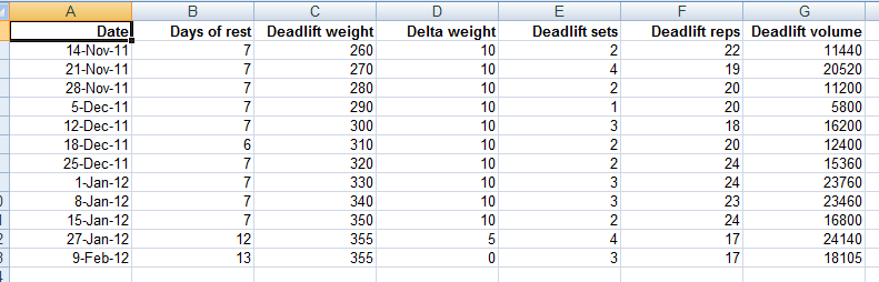
Below are four figures. The first is a table summarizing the data John obtained for his second trial. The other three are outputs from HCE, analogous to those obtained in the first trial: a table showing the coefficients of association between “Delta weight” and the other variables, two graphs (side-by-side) showing “Delta weight” against “Deadlift sets” and “Deadlift reps”, and one graph of “Delta weight” against “Days of rest”. As you can see, “Days of rest” now influences “Delta weight” very strongly. The corresponding association is a very high -0.981! The negative sign means that “Delta weight” decreases as “Days of rest” increase. This does NOT mean that rest is not important; remember, John is now operating on the right side of the J curve, with 6 or more “Days of rest”.
The last graph above suggests that taking 12 or more “Days of rest” shifted things toward the end of the supercompensation window, in fact placing John almost outside of that window at 13 “Days of rest”. Even so, there was no loss of strength, and thus probably no muscle loss. Loss of strength would be suggested by a negative “Delta weight”, which did not occur (the “Delta weight” went down to zero, at 13 “Days of rest”). The two graphs shown side-by-side suggest that 2 “Deadlift sets” seem to work just as well for John as 3 or 4, and that “Deadlift reps” in the 18-24 range also work well for John.
In this second trial, John achieved a better gain over a similar time period than in the first trial. That was a 36 percent gain from the baseline “Deadlift weight”, a gain calculated as: (355-260)/260. John started with a lower baseline than in the end of the first trial period, probably due to detraining, but achieved a final “Deadlift weight” that was likely very close to his maximum potential (at the reps used). Because of this, the 36 percent gain in the period is a lot more impressive than it looks, as it happened toward the end of a saturation curve (e.g., the far right end of a logarithmic curve).
One important thing to keep in mind is that if an HCE user identifies a nonlinear relationship of the J-curve type by inspecting the graphs like John did, in further analyses the focus should be on the right or left side of the curve by either: splitting the dataset into two, and running a separate analysis for each new dataset; or running a new trial, now sticking with a range of variation on the right or left side of the curve, as John did. The reason is that nonlinear relationships tend to distort the linear coefficients calculated by HCE, hiding a real relationship between two variables.
This is a very simplified example. Most serious bodybuilders will measure variations in a number of variables at the same time, for a number of different exercise types and formats, and for longer periods. That is, their “HealthData” sheet in HCE will be a lot more complex. They will also have multiple instances of HCE running on their computer. HCE is a collection of sheets and code that can be copied, and saved with different names. The default is “HCE_1_0.xls” or “HCE_1_0.xlsm”, depending on which version you are using. Each new instance of HCE may contain a different dataset for analysis, stored in the “HealthData” sheet.
It is strongly recommended that you keep your data in a separate set of sheets, as a backup. That is, do not store all your data in the “HealthData” sheets in different HCE instances. Also, when you copy your data into the “HealthData” sheet in HCE, copy only the values and formats, and NOT the formulas. If you copy the formulas, you may end up having some problems, as some of the cells in the “HealthData” sheet will not be storing values. I also recommend storing values for other types variables, particularly perception-based variables.
Examples of perception-based variables are: “Perceived stress”, “Perceived delayed onset muscle soreness (DOMS)”, and “Perceived non-DOMS pain”. These can be answered on Likert-type scales, such as scales going from 1 (very strongly disagree) to 7 (very strongly agree) in response to self-prepared question-statements like “I feel stressed out” (for “Perceived stress”). If you find that a variable like “Perceived non-DOMS pain” is associated with working out at a particular volume range, that may help you avoid serious injury in the future, as non-DOMS pain is not a very good sign (). You also may find that working out in the volume range that is associated with non-DOMS pain adds nothing in terms of muscle gain.
Generally speaking, I think that many people will find out that their sweet spot for muscle gain involves less frequent exercise at lower volumes than they think. Still, each individual is unique; there is no one quite like John. The relationship between “Delta weight” and “Days of rest” varies from person to person based on age; older folks generally require more rest. It also varies based on whether the person is dieting or not; less food intake leads to longer recovery periods. Women will probably see visible lower-body muscle gain, but very little visible upper-body muscle gain (in the absence of steroid use), even as they experience upper-body strength gains. Other variables of interest for both men and women may be body weight, body fat percentage, and perceived muscle tone.
Trying to hit the supercompensation window is a common denominator among HealthCorrelator for Excel (HCE) users who employ the software () to maximize muscle gain. (That is, among those who know and subscribe to the theory of supercompensation.) This post outlines what I believe is a good way of doing that while avoiding some pitfalls. The data used in the example that follows has been created by me, and is based on a real case. I disguised the data, simplified it, added error etc. to make the underlying method relatively easy to understand, and so that the data cannot be traced back to its “real case” user (for privacy).
Let us assume that John Doe is an intermediate weight training practitioner. That is, he has already gone through the beginning stage where most gains come from neural adaptation. For him, new gains in strength are a reflection of gains in muscle mass. The table below summarizes the data John obtained when he decided to vary the following variables in order to see what effects they have on his ability to increase the weight with which he conducted the deadlift () in successive exercise sessions:
- Number of rest days in between exercise sessions (“Days of rest”).
- The amount of weight he used in each deadlift session (“Deadlift weight”).
- The amount of weight he was able to add to the bar each session (“Delta weight”).
- The number of deadlift sets and reps (“Deadlift sets” and “Deadlift reps”, respectively).
- The total exercise volume in each session (“Deadlift volume”). This was calculated as follows: “Deadlift weight” x “Deadlift sets” x “Deadlift reps”.
John’s ability to increase the weight with which he conducted the deadlift in each session is measured as “Delta weight”. That was his main variable of interest. This may not look like an ideal choice at first glance, as arguably “Deadlift volume” is a better measure of total effort and thus actual muscle gain. The reality is that this does not matter much in his case, because: John had long rest periods within sets, of around 5 minutes; and he made sure to increase the weight in each successive session as soon as he felt he could, and by as much as he could, thus never doing more than 24 reps. If you think that the number of reps employed by John is too high, take a look at a post in which I talk about Doug Miller and his ideas on weight training ().
Below are three figures, with outputs from HCE: a table showing the coefficients of association between “Delta weight” and the other variables, and two graphs showing the variation of “Delta weight” against “Deadlift volume” and “Days of rest”. As you can see, nothing seems to be influencing “Delta weight” strongly enough to reach the 0.6 level that I recommend as the threshold for a “real effect” to be used in HCE analyses. There are two possibilities here: it is what it looks it is, that is, none of the variables influence “Delta weight”; or there are effects, but they do not show up in the associations table (as associations equal to or greater than 0.6) because of nonlinearity.
The graph of “Delta weight” against “Deadlift volume” is all over the place, suggesting a lack of association. This is true for the other variables as well, except “Days of rest”; the last graph above. That graph, of “Delta weight” against “Days of rest”, suggests the existence of a nonlinear association with the shape of an inverted J curve. This type of association is fairly common. In this case, it seems that “Delta weight” is maximized in the 6-7 range of “Days of rest”. Still, even varying things almost randomly, John achieved a solid gain over the time period. That was a 33 percent gain from the baseline “Deadlift weight”, a gain calculated as: (285-215)/215.
HCE, unlike WarpPLS (), does not take nonlinear relationships into consideration in the estimation of coefficients of association. In order to discover nonlinear associations, users have to inspect the graphs generated by HCE, as John did. Based on his inspection, John decided to changes things a bit, now working out on the right side of the J curve, with 6 or more “Days of rest”. That was difficult for John at first, as he was addicted to exercising at a much higher frequency; but after a while he became a “minimalist”, even trying very long rest periods.
Below are four figures. The first is a table summarizing the data John obtained for his second trial. The other three are outputs from HCE, analogous to those obtained in the first trial: a table showing the coefficients of association between “Delta weight” and the other variables, two graphs (side-by-side) showing “Delta weight” against “Deadlift sets” and “Deadlift reps”, and one graph of “Delta weight” against “Days of rest”. As you can see, “Days of rest” now influences “Delta weight” very strongly. The corresponding association is a very high -0.981! The negative sign means that “Delta weight” decreases as “Days of rest” increase. This does NOT mean that rest is not important; remember, John is now operating on the right side of the J curve, with 6 or more “Days of rest”.
The last graph above suggests that taking 12 or more “Days of rest” shifted things toward the end of the supercompensation window, in fact placing John almost outside of that window at 13 “Days of rest”. Even so, there was no loss of strength, and thus probably no muscle loss. Loss of strength would be suggested by a negative “Delta weight”, which did not occur (the “Delta weight” went down to zero, at 13 “Days of rest”). The two graphs shown side-by-side suggest that 2 “Deadlift sets” seem to work just as well for John as 3 or 4, and that “Deadlift reps” in the 18-24 range also work well for John.
In this second trial, John achieved a better gain over a similar time period than in the first trial. That was a 36 percent gain from the baseline “Deadlift weight”, a gain calculated as: (355-260)/260. John started with a lower baseline than in the end of the first trial period, probably due to detraining, but achieved a final “Deadlift weight” that was likely very close to his maximum potential (at the reps used). Because of this, the 36 percent gain in the period is a lot more impressive than it looks, as it happened toward the end of a saturation curve (e.g., the far right end of a logarithmic curve).
One important thing to keep in mind is that if an HCE user identifies a nonlinear relationship of the J-curve type by inspecting the graphs like John did, in further analyses the focus should be on the right or left side of the curve by either: splitting the dataset into two, and running a separate analysis for each new dataset; or running a new trial, now sticking with a range of variation on the right or left side of the curve, as John did. The reason is that nonlinear relationships tend to distort the linear coefficients calculated by HCE, hiding a real relationship between two variables.
This is a very simplified example. Most serious bodybuilders will measure variations in a number of variables at the same time, for a number of different exercise types and formats, and for longer periods. That is, their “HealthData” sheet in HCE will be a lot more complex. They will also have multiple instances of HCE running on their computer. HCE is a collection of sheets and code that can be copied, and saved with different names. The default is “HCE_1_0.xls” or “HCE_1_0.xlsm”, depending on which version you are using. Each new instance of HCE may contain a different dataset for analysis, stored in the “HealthData” sheet.
It is strongly recommended that you keep your data in a separate set of sheets, as a backup. That is, do not store all your data in the “HealthData” sheets in different HCE instances. Also, when you copy your data into the “HealthData” sheet in HCE, copy only the values and formats, and NOT the formulas. If you copy the formulas, you may end up having some problems, as some of the cells in the “HealthData” sheet will not be storing values. I also recommend storing values for other types variables, particularly perception-based variables.
Examples of perception-based variables are: “Perceived stress”, “Perceived delayed onset muscle soreness (DOMS)”, and “Perceived non-DOMS pain”. These can be answered on Likert-type scales, such as scales going from 1 (very strongly disagree) to 7 (very strongly agree) in response to self-prepared question-statements like “I feel stressed out” (for “Perceived stress”). If you find that a variable like “Perceived non-DOMS pain” is associated with working out at a particular volume range, that may help you avoid serious injury in the future, as non-DOMS pain is not a very good sign (). You also may find that working out in the volume range that is associated with non-DOMS pain adds nothing in terms of muscle gain.
Generally speaking, I think that many people will find out that their sweet spot for muscle gain involves less frequent exercise at lower volumes than they think. Still, each individual is unique; there is no one quite like John. The relationship between “Delta weight” and “Days of rest” varies from person to person based on age; older folks generally require more rest. It also varies based on whether the person is dieting or not; less food intake leads to longer recovery periods. Women will probably see visible lower-body muscle gain, but very little visible upper-body muscle gain (in the absence of steroid use), even as they experience upper-body strength gains. Other variables of interest for both men and women may be body weight, body fat percentage, and perceived muscle tone.
Labels:
exercise injuries,
HCE,
muscle gain,
resistance exercise,
statistics,
strength training,
supercompensation,
warppls
Subscribe to:
Posts (Atom)