If your NEAT is low, maybe you should chill

I wrote most of this post a while ago, and then forgot about it. The recent blogosphere storm of comments regarding cold-induced thermogenesis caught me by surprise (), and provided a motivation to get this post out. Contrary to popular perception, I guess, cold-induced thermogenesis is an extensively researched topic. Some reasonably well cited references are linked here.

Let us backtrack a bit. When people say that they want to lose weight, usually what they really want is to lose is body fat. However, they frequently do things that make them lose what they do not want – muscle glycogen, water, and even some muscle protein. Physical activity in general depletes muscle glycogen; even aerobic physical activity.

Walking, for example, depletes muscle glycogen; but slowly, and proportionally to how fast one walks. Weight training and sprints deplete muscle glycogen much faster. Whatever depletes muscle glycogen also lowers the amount of water stored in myocytes (muscle cells), effectively reducing muscle mass. Depleted muscle glycogen needs to be replenished; protein and carbohydrates are the sources. If you deplete muscle glycogen through strength training, this will provide a strong stimulus for glycogen replenishment and thus muscle growth, even beyond the original level – a phenomenon called supercompensation ().

In conjunction with strength training, situations in which one burns mostly fat, and very little glycogen, should be at the top of the list for those wishing to lose weight by losing body fat and nothing else. These are not very common though. One example is nonexercise activity thermogenesis (NEAT), or heat generation from nonexercise activities such as fidgeting (). There is a great deal of variation in NEAT across individuals; for some it is high, for others it is annoyingly low.

Walking slowly is almost as good as NEAT for body fat burning, when done in conjunction with strength training. Up the pace a bit though, and you’ll be burning more muscle glycogen. But if you walk slowly you don’t burn that much body fat per unit of time. If you walk a bit faster you’ll burn more fat, but also more glycogen. C’mon, there is no way to win in this game!

This is why being physically active, in a “non-exercise way”, seems to be so important for health; together with strength training, limiting calorie intake, and all the while having a nutritious diet. These are not very common things in modern urban environments. Long term, there isn’t a lot of margin for error. It is ultimately a game of small numbers in the short term, played over long periods of time.

But there is an alternative if your NEAT is low – just chill. That is, another situation in which one can burn mostly fat, and very little glycogen, is exposure to mildly cold temperatures, but above the level that induces shivering (mild cold: 16 degrees Celsius or so; about 60 degrees Fahrenheit). Shivering in general, and particularly intense shivering, is associated with levels of muscle activity that would induce glycogen depletion () (). If muscle glycogen depletion happens while one is fasting, liver glycogen will be used to replenish muscle glycogen, and also to supply the needs of the brain – which is always hungry for glucose.

As the liver glycogen tank goes down beyond a certain point, and no protein or carbohydrates are eaten, the body will use amino acids from muscle to produce glucose. Muscle glycogen will be locked until it is needed. Interesting eh!? The body sacrifices muscle protein but doesn’t tap into muscle glycogen, which is only used to fuel violent muscle contractions. We are talking about fight-or-flight responses here. From an evolutionary perspective, sacrificing some muscle beats losing a lot of it to a predator any day.

Cold-induced thermogenesis is a very interesting phenomenon. The figure below, where open circles represent lean and closed circles obese folks, shows that it leads to different responses in lean and obese folks, and also that it presents a lot of variation across different individuals (like NEAT). This type of thermogenesis actually seems to be strongly associated with an increase in NEAT (); although it seems to also be associated with futile cycles used by the body to generate heat without any movement, as in thermogenesis during hibernation in certain animals () (). Having more brown fat as an adult, or being able to make brown fat more easily, is associated with more cold-induced thermogenesis; and also with a lower obesity risk.

In fact, cold-induced thermogenesis leads to an increase in energy expenditure that is comparable with that of another major energy sinkhole – overfeeding () (). Unlike overfeeding though, cold-induced thermogenesis does not require calories to go in. And, no, you don’t burn more than you take in with overfeeding.

How can one burn fat via cold-induced thermogenesis? Here are some ideas. Set the home thermostat to a mildly cold temperature in the winter (this will also save you some money). When it is a little cooler than normal, don’t wear heavy clothes. Take mildly cold showers, or end a warm shower with some mildly cold water.

What about more extreme cold exposure? It should be no surprise that one would feel pretty good after a dip in ice-cold water; that is, if the person does not suffer from a glycogen storage disease (e.g., McArdle's disease). At least in theory, that type of cold exposure should induce whole-body muscle glycogen depletion, just like an intense whole-body exercise session, with the resulting hormonal changes ().

Growth hormone should be up after that, perhaps for hours. Done right after weight training, or intense exercise, it may have a boosting effect on the hormonal response. But if you do that in the recovery phase (e.g., several hours after the weight training session), it should impair muscle recovery. It would be a bit like doing another strength training session, when the body is trying to recover from the previous one.

Finding your sweet spot for muscle gain with HCE

In order to achieve muscle gain, one has to repeatedly hit the “supercompensation” window, which is a fleeting period of time occurring at some point in the muscle recovery phase after an intense anaerobic exercise session. The figure below, from Vladimir Zatsiorsky’s and William Kraemer’s outstanding book Science and Practice of Strength Training () provides an illustration of the supercompensation idea. Supercompensation is covered in more detail in a previous post ().

Trying to hit the supercompensation window is a common denominator among HealthCorrelator for Excel (HCE) users who employ the software () to maximize muscle gain. (That is, among those who know and subscribe to the theory of supercompensation.) This post outlines what I believe is a good way of doing that while avoiding some pitfalls. The data used in the example that follows has been created by me, and is based on a real case. I disguised the data, simplified it, added error etc. to make the underlying method relatively easy to understand, and so that the data cannot be traced back to its “real case” user (for privacy).

Let us assume that John Doe is an intermediate weight training practitioner. That is, he has already gone through the beginning stage where most gains come from neural adaptation. For him, new gains in strength are a reflection of gains in muscle mass. The table below summarizes the data John obtained when he decided to vary the following variables in order to see what effects they have on his ability to increase the weight with which he conducted the deadlift () in successive exercise sessions:
    - Number of rest days in between exercise sessions (“Days of rest”).
    - The amount of weight he used in each deadlift session (“Deadlift weight”).
    - The amount of weight he was able to add to the bar each session (“Delta weight”).
    - The number of deadlift sets and reps (“Deadlift sets” and “Deadlift reps”, respectively).
    - The total exercise volume in each session (“Deadlift volume”). This was calculated as follows: “Deadlift weight” x “Deadlift sets” x “Deadlift reps”.

John’s ability to increase the weight with which he conducted the deadlift in each session is measured as “Delta weight”. That was his main variable of interest. This may not look like an ideal choice at first glance, as arguably “Deadlift volume” is a better measure of total effort and thus actual muscle gain. The reality is that this does not matter much in his case, because: John had long rest periods within sets, of around 5 minutes; and he made sure to increase the weight in each successive session as soon as he felt he could, and by as much as he could, thus never doing more than 24 reps. If you think that the number of reps employed by John is too high, take a look at a post in which I talk about Doug Miller and his ideas on weight training ().

Below are three figures, with outputs from HCE: a table showing the coefficients of association between “Delta weight” and the other variables, and two graphs showing the variation of “Delta weight” against “Deadlift volume” and “Days of rest”. As you can see, nothing seems to be influencing “Delta weight” strongly enough to reach the 0.6 level that I recommend as the threshold for a “real effect” to be used in HCE analyses. There are two possibilities here: it is what it looks it is, that is, none of the variables influence “Delta weight”; or there are effects, but they do not show up in the associations table (as associations equal to or greater than 0.6) because of nonlinearity.

The graph of “Delta weight” against “Deadlift volume” is all over the place, suggesting a lack of association. This is true for the other variables as well, except “Days of rest”; the last graph above. That graph, of “Delta weight” against “Days of rest”, suggests the existence of a nonlinear association with the shape of an inverted J curve. This type of association is fairly common. In this case, it seems that “Delta weight” is maximized in the 6-7 range of “Days of rest”. Still, even varying things almost randomly, John achieved a solid gain over the time period. That was a 33 percent gain from the baseline “Deadlift weight”, a gain calculated as: (285-215)/215.

HCE, unlike WarpPLS (), does not take nonlinear relationships into consideration in the estimation of coefficients of association. In order to discover nonlinear associations, users have to inspect the graphs generated by HCE, as John did. Based on his inspection, John decided to changes things a bit, now working out on the right side of the J curve, with 6 or more “Days of rest”. That was difficult for John at first, as he was addicted to exercising at a much higher frequency; but after a while he became a “minimalist”, even trying very long rest periods.

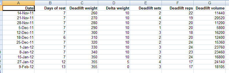
Below are four figures. The first is a table summarizing the data John obtained for his second trial. The other three are outputs from HCE, analogous to those obtained in the first trial: a table showing the coefficients of association between “Delta weight” and the other variables, two graphs (side-by-side) showing “Delta weight” against “Deadlift sets” and “Deadlift reps”, and one graph of “Delta weight” against “Days of rest”. As you can see, “Days of rest” now influences “Delta weight” very strongly. The corresponding association is a very high -0.981! The negative sign means that “Delta weight” decreases as “Days of rest” increase. This does NOT mean that rest is not important; remember, John is now operating on the right side of the J curve, with 6 or more “Days of rest”.

The last graph above suggests that taking 12 or more “Days of rest” shifted things toward the end of the supercompensation window, in fact placing John almost outside of that window at 13 “Days of rest”. Even so, there was no loss of strength, and thus probably no muscle loss. Loss of strength would be suggested by a negative “Delta weight”, which did not occur (the “Delta weight” went down to zero, at 13 “Days of rest”). The two graphs shown side-by-side suggest that 2 “Deadlift sets” seem to work just as well for John as 3 or 4, and that “Deadlift reps” in the 18-24 range also work well for John.

In this second trial, John achieved a better gain over a similar time period than in the first trial. That was a 36 percent gain from the baseline “Deadlift weight”, a gain calculated as: (355-260)/260. John started with a lower baseline than in the end of the first trial period, probably due to detraining, but achieved a final “Deadlift weight” that was likely very close to his maximum potential (at the reps used). Because of this, the 36 percent gain in the period is a lot more impressive than it looks, as it happened toward the end of a saturation curve (e.g., the far right end of a logarithmic curve).

One important thing to keep in mind is that if an HCE user identifies a nonlinear relationship of the J-curve type by inspecting the graphs like John did, in further analyses the focus should be on the right or left side of the curve by either: splitting the dataset into two, and running a separate analysis for each new dataset; or running a new trial, now sticking with a range of variation on the right or left side of the curve, as John did. The reason is that nonlinear relationships tend to distort the linear coefficients calculated by HCE, hiding a real relationship between two variables.

This is a very simplified example. Most serious bodybuilders will measure variations in a number of variables at the same time, for a number of different exercise types and formats, and for longer periods. That is, their “HealthData” sheet in HCE will be a lot more complex. They will also have multiple instances of HCE running on their computer. HCE is a collection of sheets and code that can be copied, and saved with different names. The default is “HCE_1_0.xls” or “HCE_1_0.xlsm”, depending on which version you are using. Each new instance of HCE may contain a different dataset for analysis, stored in the “HealthData” sheet.

It is strongly recommended that you keep your data in a separate set of sheets, as a backup. That is, do not store all your data in the “HealthData” sheets in different HCE instances. Also, when you copy your data into the “HealthData” sheet in HCE, copy only the values and formats, and NOT the formulas. If you copy the formulas, you may end up having some problems, as some of the cells in the “HealthData” sheet will not be storing values. I also recommend storing values for other types variables, particularly perception-based variables.

Examples of perception-based variables are: “Perceived stress”, “Perceived delayed onset muscle soreness (DOMS)”, and “Perceived non-DOMS pain”. These can be answered on Likert-type scales, such as scales going from 1 (very strongly disagree) to 7 (very strongly agree) in response to self-prepared question-statements like “I feel stressed out” (for “Perceived stress”). If you find that a variable like “Perceived non-DOMS pain” is associated with working out at a particular volume range, that may help you avoid serious injury in the future, as non-DOMS pain is not a very good sign (). You also may find that working out in the volume range that is associated with non-DOMS pain adds nothing in terms of muscle gain.

Generally speaking, I think that many people will find out that their sweet spot for muscle gain involves less frequent exercise at lower volumes than they think. Still, each individual is unique; there is no one quite like John. The relationship between “Delta weight” and “Days of rest” varies from person to person based on age; older folks generally require more rest. It also varies based on whether the person is dieting or not; less food intake leads to longer recovery periods. Women will probably see visible lower-body muscle gain, but very little visible upper-body muscle gain (in the absence of steroid use), even as they experience upper-body strength gains. Other variables of interest for both men and women may be body weight, body fat percentage, and perceived muscle tone.

The theory of supercompensation: Strength training frequency and muscle gain

Moderate strength training has a number of health benefits, and is viewed by many as an important component of a natural lifestyle that approximates that of our Stone Age ancestors. It increases bone density, muscle mass, and improves a number of health markers. Done properly, it may decrease body fat percentage.

Generally one would expect some muscle gain as a result of strength training. Men seem to be keen on upper-body gains, while women appear to prefer lower-body gains. Yet, many people do strength training for years, and experience little or no muscle gain.

Paradoxically, those people experience major strength gains, both men and women, especially in the first few months after they start a strength training program. However, those gains are due primarily to neural adaptations, and come without any significant gain in muscle mass. This can be frustrating, especially for men. Most men are after some noticeable muscle gain as a result of strength training. (Whether that is healthy is another story, especially as one gets to extremes.)

After the initial adaptation period, of “beginner” gains, typically no strength gains occur without muscle gains.

The culprits for the lack of anabolic response are often believed to be low levels of circulating testosterone and other hormones that seem to interact with testosterone to promote muscle growth, such as growth hormone. This leads many to resort to anabolic steroids, which are drugs that mimic the effects of androgenic hormones, such as testosterone. These drugs usually increase muscle mass, but have a number of negative short-term and long-term side effects.

There seems to be a better, less harmful, solution to the lack of anabolic response. Through my research on compensatory adaptation I often noticed that, under the right circumstances, people would overcompensate for obstacles posed to them. Strength training is a form of obstacle, which should generate overcompensation under the right circumstances. From a biological perspective, one would expect a similar phenomenon; a natural solution to the lack of anabolic response.

This solution is predicted by a theory that also explains a lack of anabolic response to strength training, and that unfortunately does not get enough attention outside the academic research literature. It is the theory of supercompensation, which is discussed in some detail in several high-quality college textbooks on strength training. (Unlike popular self-help books, these textbooks summarize peer-reviewed academic research, and also provide the references that are summarized.) One example is the excellent book by Zatsiorsky & Kraemer (2006) on the science and practice of strength training.

The figure below, from Zatsiorsky & Kraemer (2006), shows what happens during and after a strength training session. The level of preparedness could be seen as the load in the session, which is proportional to: the number of exercise sets, the weight lifted (or resistance overcame) in each set, and the number of repetitions in each set. The restitution period is essentially the recovery period, which must include plenty of rest and proper nutrition.

Note that toward the end there is a sideways S-like curve with a first stretch above the horizontal line and another below the line. The first stretch is the supercompensation stretch; a window in time (e.g., a 20-hour period). The horizontal line represents the baseline load, which can be seen as the baseline strength of the individual prior to the exercise session. This is where things get tricky. If one exercises again within the supercompensation stretch, strength and muscle gains will likely happen. (Usually noticeable upper-body muscle gain happens in men, because of higher levels of testosterone and of other hormones that seem to interact with testosterone.) Exercising outside the supercompensation time window may lead to no gain, or even to some loss, of both strength and muscle.

Timing strength training sessions correctly can over time lead to significant gains in strength and muscle (see middle graph in the figure below, also from Zatsiorsky & Kraemer, 2006). For that to happen, one has not only to regularly “hit” the supercompensation time window, but also progressively increase load. This must happen for each muscle group. Strength and muscle gains will occur up to a point, a point of saturation, after which no further gains are possible. Men who reach that point will invariably look muscular, in a more or less “natural” way depending on supplements and other factors. Some people seem to gain strength and muscle very easily; they are often called mesomorphs. Others are hard gainers, sometimes referred to as endomorphs (who tend to be fatter) and ectomorphs (who tend to be skinnier).

It is not easy to identify the ideal recovery and supercompensation periods. They vary from person to person. They also vary depending on types of exercise, numbers of sets, and numbers of repetitions. Nutrition also plays a role, and so do rest and stress. From an evolutionary perspective, it would seem to make sense to work all major muscle groups on the same day, and then do the same workout after a certain recovery period. (Our Stone Age ancestors did not do isolation exercises, such as bicep curls.) But this will probably make you look more like a strong hunter-gatherer than a modern bodybuilder.

To identify the supercompensation time window, one could employ a trial-and-error approach, by trying to repeat the same workout after different recovery times. Based on the literature, it would make sense to start at the 48-hour period (one full day of rest between sessions), and then move back and forth from there. A sign that one is hitting the supercompensation time window is becoming a little stronger at each workout, by performing more repetitions with the same weight (e.g., 10, from 8 in the previous session). If that happens, the weight should be incrementally increased in successive sessions. Most studies suggest that the best range for muscle gain is that of 6 to 12 repetitions in each set, but without enough time under tension gains will prove elusive.

The discussion above is not aimed at professional bodybuilders. There are a number of factors that can influence strength and muscle gain other than supercompensation. (Still, supercompensation seems to be a “biggie”.) Things get trickier over time with trained athletes, as returns on effort get progressively smaller. Even natural bodybuilders appear to benefit from different strategies at different levels of proficiency. For example, changing the workouts on a regular basis seems to be a good idea, and there is a science to doing that properly. See the “Interesting links” area of this web site for several more focused resources of strength training.

Reference:

Zatsiorsky, V., & Kraemer, W.J. (2006). Science and practice of strength training. Champaign, IL: Human Kinetics.